What’s your interpretation? – November and December, 1999
What’s your interpretation? |
 This example deals with a herd experiencing low farrowing
rate (74%). These data were taken from 198 PigCHAMP records. The
herd had recently begun using artificial insemination (AI) and
so I examined the relationship between farrowing rate and AI.
The herd is also in expansion mode and 32% of the records were
for gilts. Does this herd have a problem with AI technology?
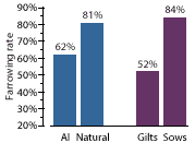
As you can see from the figure on the front cover, the AI breedings resulted in a 62% farrowing rate compared to 81% for natural breedings. Gilts had a 52% farrowing rate compared to a 84% farrowing rate for sows. Therefore, the producer appears to have trouble with AI and with gilts.
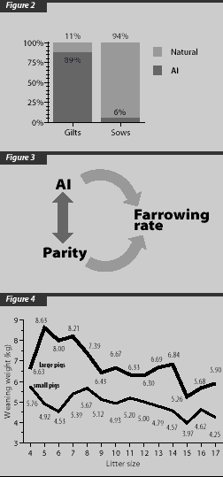
 In Figure 2, you can see that the producer is using
AI primarily for gilts and natural mating for sows. Since 89%
of gilts were bred by AI and only 6% of sows were bred by AI,
there is no way to separate the effect of the AI from the effect
of being a gilt.
This three-way relationship (Figure 3) between variables is called confounding. Confounding is not a biological phenomenon. It is data set dependent. Even so, when confounding is present in one data set, it may be present in other data sets and therefore it is wise to test for the presence of confounding. Typical confounding variables include gender, age, parity and pen.
Confounding variables are related to both the causative factor and the outcome variable. In this case, parity is associated with both low farrowing rate and the use of AI. Similarly, AI also associated with low farrrowing rate. There is always this triangle of association.
To analyze for a potential confounding variable you must collect data on potential confounding factors and then include those factors in a multivariate analysis. In our example, we would examine the relationship between farrowing rate and AI, after "controlling" for parity.
Figure 4 illustrates another relationship between variables called interaction. Unlike confounding, interaction is a biological phenomenon. There must be a biological explanation for this relationship and the interaction relationship is expected to occur in all data sets.
Interaction occurs when the relationship between the causative factor and the outcome is dependent on a third factor. In our example, the relationship between the size of the litter nursing the sow and the weaning weight of the pig differs for small and large pigs. As we increase the number of pigs nursing the sow, weaning weights decrease. Although this phenomenon is true for all sizes of pigs, the impact on the weaning weights of large pigs is greater that the impact on small pigs. In other words, small pigs can tolerate large litter sizes more than large pigs can.
Other examples of interaction include: the association between lactation feed intake and subsequent weaning-to-breeding interval may change according to parity. Parity is the interaction variable. The relationship between lactation intake and weaning-to-breeding interval may be different for young parity sows than older parity sows.
To test for interaction, we create an interaction variable by multiplying the two variables of interest by one another. In our example, we multiply birth weight by litter size. In the multiple regression equation, we include the simple effects; birth weight and litter size and also include the (birth weight x litter size ) variable. If there is interaction, the P value for the interaction term will be <.05.
–Submitted by Cate Dewey