Wnat’s your interpretation? — January 1999
What’s your interpretation? |
 |
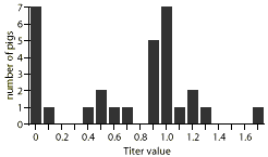
This figure shows the frequency distribution of results from an ELISA test of antibodies to porcine reproductive and respiratory syndrome virus (PRRSV). Blood samples were collected from 30 pigs in a herd. Can you calculate average titer and its standard deviation? |
 Standard deviation and frequency
distribution
Cases
- The mean titer of the data shown in the Figure on the cover is 0.66, with a standard deviation (SD) of 0.47.
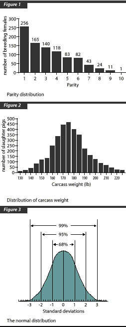
- Figure 1 is the parity distribution of a breeding herd with 923 females. Mean parity is 3.2, with an SD of 2.1.
- Figure 2 is the distribution of carcass weight from 3403 pigs. Mean weight is 80.8 kg (178.0 lb) with an SD of 7.6 kg (16.7 lb).
Interpretation
Standard deviation describes the variation of the variable of the data–on the average, how much individual values differ from the mean. Calculation of SD is based on data with a normal distribution: a bell-shaped curve (Figure 3). The value at 0 in Figure 3 is the mean of the data. When the data are normally distributed, approximately 68% of observations fall between -1 and 1 standard deviations from the mean; 95% of observations fall between -2 and 2 standard deviations from the mean; and 99% of observations fall between -3 and 3 standard deviations from the mean.
According to this principle,
- 68% of carcasses in Figure 2 are between 73.2 and 88.4 kg (161-194 lb),
- 95% of carcasses are between 65.5 and 96.0 kg (144-211 lb), and
- 99% of carcasses are between 58.0 and 103.6 kg (130-228 lb).
If we use the same method to describe the data in Figure 1:
- 68% of females will fall between parities 1.1 and 5.3,
- 95% of females will fall between parities -1.0 and 7.4, and
- 99% of females will fall between parities -3.1 and 9.5.
It is obvious that the data are not well described by SD, because it is not possible to have negative (-) parity animals. The problem in this case is that the data are not normally distributed/as illustrated by the non-normal distribution curve.
In the real world, one may not calculate the mean titer of an ELISA test. It is common to use a cutoff value (e.g., 0.4) to group data into positives and negatives. Samples with titers less than the cutoff value are categorized as negative and those with titers equal to or larger than the cutoff value are categorized as positive. This case demonstrates the change of a continuous variable into a categorical variable.
Summary
It is common to use standard deviation to describe variation of the data that are normally distributed. It is not meaningful to use standard deviation when data are not normally distributed.
This page last updated .