What's your interpretation?	March and April, 1998

This month, "What's your interpretation?" has been written by Bob Morrison, Vickie King, and Ruth Cronje.

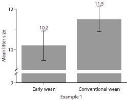
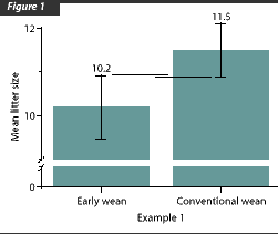
This figure (Figure 1) represents data from a hypothetical example. It compares mean litter size in a treatment group that was weaned at 21 days versus a treatment group that was weaned at 7 days. In this hypothetical example, litter size significantly differed between the two groups (P < .05). Notice that the 95% confidence intervals (95% CI) overlap. How can the 95%CI overlap for values that differ statistically?

As you may have noticed, SHAP has begun to report variation of the data sampled (i.e., the spread of data around the mean) as 95% confidence intervals (95%CI), rather than as standard deviations (SD). Because 95% CI is calculated with a formula that incorporates sample size and variation, it provides an estimate of the precision of the population mean. That is, if the population was repeatedly sampled, the mean of the sample would fall within the 95% CI, 95 times out of 100. Although when comparing two samples and their respective CIs it is convenient to look for overlap to get a quick impression of the statistical difference between the means, the CI bars do not tell us the statistical significance of the difference. Confidence intervals and P values are two different pieces of information, each designed to tell us something different about the data. In this month's "What's your interpretation," we'll be discussing the relative meaning of the P value and the confidence interval.

In hypothetical Example 1 (Figure 1), litter size for early-weaned (EW) sows ranged from 7-13, and for conventionally weaned (CW) sows, ranged from 7-14. The mean for the EW group was 10.2 and for the CW group was 11.5.

Our first step is to analyze these data is using Bartlett's test to determine whether the variation in the data for the CW sows differed significantly from that of the EW sows. In Example 1, we discovered that the variation did not differ statistically between the two groups. This allowed us to pool the variance in subsequent statistical analysis, using one value for variation for both CW and EW sows.

But determining the statistical difference of the variation in groups is not the only thing we are statistically interested in. We must also test the null hypothesis that weaning age did NOT have an effect on litter size in our example. To test our null hypothesis, we need to determine whether the mean litter size of the EW group (10.2 pigs) and the mean litter size of the CW group (11.5 pigs) are different (Figure 1). That is, is weaning age a true factor influencing litter size or do the means differ because our observations were the result of chance variation ("noise")? Our next step, then, is to perform Student's t-test. We found that the means in litter size for these two groups of sows differed significantly (P<.05)--which means that there is at least a 19 in 20 chance that our observations are biologically "real" and not merely "noise"--a degree of probability acceptable within most scientific communities. With this result, we reject the null hypothesis, and are justified in concluding that, in this example, weaning age was significantly associated with litter size.

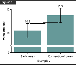
Let's compare the results of Example 1 to another hypothetical example (Example 2), investigating the same hypothesis. In Example 2, we again included 80 sows in the CW group and 80 in the EW group. The means we observed were the same as those observed in Example 1 for both groups: 10.2 pigs for the EW group and 11.5 pigs for the CW group (Figure 2). In Example 2, however, although the variability in the CW group remained the same as in Example 1, the variability in the EW group decreased. This decrease in variability at the same sample size is reflected in the slightly shorter 95%CI for the CW group in Figure 2. In this case, the 95% CI do not overlap, but again after we use the Student's t-test to compare the means of the EW and CW groups, the differences in mean litter sizes prove to be statistically different.

Implications

When interpreting the results of experimental data, it is important to understand that the 95%CI and P values are not the same statistical measure. Each is telling us something slightly different about the data we are looking at, and each is necessary for a full understanding of the significance of experimental results. Here are a few rules of thumb to keep in mind:

• If the 95%CI DO NOT overlap, you can always be certain that P <.05, and that the difference in treatment groups is "significant"--i.e., that it is a "real" difference and probably repeatable.
• If the 95%CI DO overlap, it is not automatically safe to conclude that "the difference is not significant." This is because 95%CI show ONLY the variation around the mean within a given treatment group and in no way reflect a measure of the likelihood that the difference in means between or among treatment groups (for which different statistical tests need to be applied) is a chance phenomenon (i.e., P<.05).

For this reason, we shall continue to provide both 95%CI and P values for the data we report in SHAP.