What’s your interpretation? |
Non refereed |
What does a mean mean?
Eric Bush, DVM, MS
USDA:APHIS:VS-CNAHS, 2150 Centre Ave, Building B-2E7, Fort Collins, CO 80526-8117; Tel: 970-494-7260; Fax: 970-494-7229; http://www.aphis.usda.gov/vs/ceah/cahm/Swine/swine.htm
Cite as: Bush E. What does a mean mean?. J Swine Health Prod. 2004;12(4):214-215.
When serological data from pro- duction systems are evaluated, the mean is probably the most commonly used calculation. This is because the mean provides a handy measure of ‘central tendency’ and therefore serves as a very succinct summary of a large number of data points. It is calculated by adding up the values of all observations (xi) and then dividing by the number of observations (n). In essence, it describes where the center of gravity is for a distribution of data points. Other measures of central tendency include the median and mode. The median is also a dividing point, but it ignores the value (or weight) of each observation. It is calculated by lining up all the observations from smallest to largest and determining the value of the middle observation. For the median, half of the observations have a value smaller than the median (or 50th percentile) and half have a value greater than the median.1 The mode is simply the most common value observed.
 Conveniently, when data are normally distributed (ie, the data points have a
symmetric bell shape), the mean, median, and mode are all the same value. Thus,
they each represent the central point, the most typical value, and the center of gravity for
a symmetrical distribution. Unfortunately, real biological data are not always
distributed normally, and the mean may mislead the undiscerning reader. Since the mean
is calculated by totaling the values of all observations, extremely high or low
values can greatly influence the mean. This is especially true when there are relatively
few observations, but even in large data sets there may be a tendency toward many
extreme values (either large or small), and these values pull the distribution in
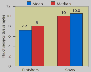
their direction (ie, skew the data). For example, in the figure on the back cover, since
many breeding herds have a large number of
Mycoplasma hyopneumoniae-positive sows
or gilts,2 the data are not a perfect fit with
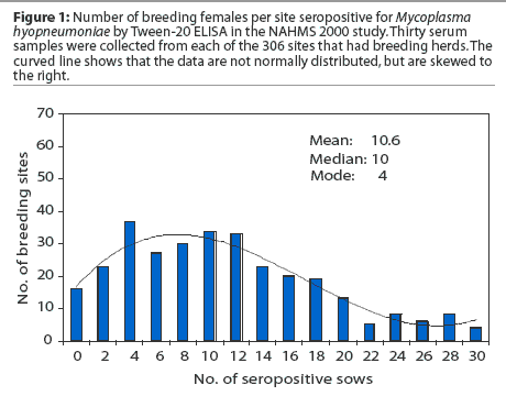
the normal distribution, but are skewed to the right of the median (mean of 10.6
versus median of 10). Thus, knowing both the mean and median may sometimes
provide a clue to the direction in which the data
is skewed. When one evaluates a histogram of the breeding herd data (Figure 1), one
can more readily observe this skew.
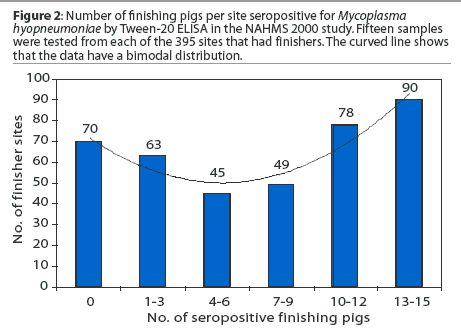
Assuming the way the data is skewed by just evaluating the mean and median presumes that the data at least approximate a normal distribution. In the case of the finishing herd, this may be a dangerous assumption. For the finishing data in the back cover figure, looking at the mean (7.2) and median (8) might lead one to conclude that the data are skewed slightly to the left. One might also assume that the most typical number of positive finisher samples would be around 7 to 8 of 15 (50% positive). The data are skewed, but relatively few farms had around 50% of finishers positive. This can be seen in Figure 2, which is a histogram of the number of positive samples. Finishing herds tended to be either "negative" (three or fewer positive samples) or mostly positive (75 to 100% of finishers positive). In other words, there are two modes or most frequent values (0 and 12). When data has a bimodal distribution, the mean is not the most typical value and will be very different from the mode.
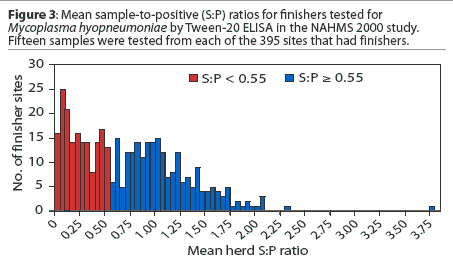
A variety of underlying processes can give rise to a bimodal distribution of data. One example is the existence of two distinct populations with overlapping distributions. The mean sample-to-positive (S:P) ratio was calculated for each finishing herd. Figure 3 shows the frequency distribution of the mean herd S:P ratios and divides the sites into two populations – herds with a mean S:P ratio < 0.55 and those with a mean S:P ratio >= 0.55. Figure 4 shows that the bimodal distribution of Figure 2 consists of two distinct populations: sites with ‘low’ mean S:P ratios and sites with ‘high’ mean S:P ratios.3 The mean numbers of seropositives for these two populations are 1.5 and 11.4 respectively.
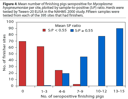
In summary, never interpret a mean value without knowing the underlying distribution (or the sample size). It is always a good practice to generate a histogram to determine whether the data are normally distributed, bimodal, or skewed. If the data approximate a normal distribution (bell shape), then the mean will be equivalent to the median and mode. With skewed data, the mean cannot be interpreted as the most central point (median), and with data distributed bimodally, the mean cannot be interpreted as the most typical value (mode). You know what I mean?
References
*1. Erlandson KR, Thacker BJ, Bush EJ. Mycoplasma hyopneumoniae seroprevalence and control strategies on farms participating in the NAHMS Swine 2000 survey. Proc AASV. Orlando, Florida. 2003:31-34. Available on AASV CD-ROM
2. Levonen K, Sihvo E, Veijalainen P. Comparison of two commercial enzyme-linked immunosorbent assays for the detection of antibodies against Mycoplasma hyopneumoniae and correlation with herd status. J Vet Diagn Invest. 1999;11:547-549.
*3. Thacker EL. Mycoplasma diagnosis and immunity. Proc AASV. Nashville, Tennessee. 2001:467. Available on AASV CD-ROM
*Non-refereed references.